Understanding edge- and line-based segmentation
Understanding edge- and line-based segmentation
ROBERT BELKNAP
Segmentation techniques that extract boundaries or edges attempt to identify points in an image where there are discontinuities or differences between pixel values. That is, edges are placed where changes of gray-level intensity occur in the image. The assumption is made that these changes occur in the data at the boundary between the objects of interest.
The output of edge segmentation schemes can be
X and Y gradient--Two images are used to represent the detected edges, one in the x (horizontal) direction and one in the y (vertical) direction.
Gradient strength and direction-- A pair of images is produced. One holds the gradient strength at every pixel in the image, and the other holds the direction.
Binary edge map--The output image is set to all zeros except at locations where edges are found, which are set to ones or binary true.
Edgel representation--Data structures called edge elements are used to hold single units of edge strength and direction. Sometimes the gradient strength/ direction image pair is referred to as an edgel representation.
The most prevalent edge-segmentation techniques are mask-based averaging edge detectors such as the Sobel, Prewitt, and Roberts operators. The approach that these operators use is to locate points in the image where significant gradient changes are occurring. They use pixel-neighborhood averaging, as defined by the masks or kernels, to reduce the effects of noise. In a sense, they transform an input image into an edge image by boosting the output where changes are occurring (edges) and suppressing them where little or no change is occurring (background).
The operators perform their functionality by differencing. That is, their output is some function of the difference between a pixel`s intensity value and the values of its neighbors, as defined by the pixel selection and weighting masks used in implementing the function. In essence, this is a discrete form of a derivative function, a computation that derives a measure of rate of change, which is greatest around the edges in the image.
Many masks have been devised for edge detection, and most have been developed using some kind of optimality criteria such as sensitivity--the ability to detect weak or low contrast edges; elimination of false edges--the ability to reject noise; and accuracy--the exactness to which the edge magnitude and/or direction is computed.
One similarity between all the mask-based operators is that they come in sets, as most masks can compute a difference in one direction only. In this case, the minimum number of masks needed to compute the edge is two. Almost always, one mask computes the difference in the x direction, while the other computes the change in the y direction. These masks are convolved with the image to produce a set of output images: one for the rate of change in the x direction, called dx, and one for the rate of change in the y direction, called dy (see Vision Systems Design, June 1998, p. 20).
Using trigonometry, the edge magnitude and direction can be calculated as
Magnitude = SQRT (dx2 + dy2)
Direction = tan-1 (dy/dx)
This calculation is used to transform the x and y difference into the magnitude and direction pair (see Fig. 1 on p. 27). An exception to this is the Laplacian operator, which combines the dx and dy computations into one convolution kernel and produces an edge-strength image. However, in doing so, the edge-direction information is lost (it is an isotropic operator).
Compass masks are used whenever greater accuracy is needed or there is a need to compute a set of directional edge images that can be used for further analysis, such as texture computation. These masks take their name from the points of a compass and have their weights oriented in such a manner as to calculate the gradients in one of the following compass directions: N, NE, E, SE, S, SW, W, and NW.
If a single edge representation is needed, nonmaximal suppression is used to select the strongest response. That is, an output image is created in which the pixels are set to the highest value calculated by the eight masks. The direction is taken from the orientation of the mask that produces this maximal value. Compass masks reduce the inaccuracies caused by the averaging effects of convolution kernels, and the directional error is bounded to
360º 8 2 = 22.5°
That is, there are eight masks to measure a total of 360° of direction, and the resulting true direction will be at most halfway between one of the measured directions.
To create a set of compass masks, take a favorite edge operator and rotate it in 45° increments to create all eight masks. In actuality, you only need to compute and apply four of these masks, because the sign of the result will indicate the direction (for example, a negative result from the NE mask indicates a SW direction). A word of caution, however; in some masks, such as the Sobel, the kernel weights are selected based on the distance between the centers of the central-to-neighborhood pixels. These distances can change when the mask is rotated, and if this is not compensated, some of the directional masks will create stronger responses, thereby biasing the results. The result of the application of mask-based convolution operators is not a segmentation, and most often, the application of these operators is followed by further processing such as nonmaximal suppression, thresholding, and edge thinning (see Vision Systems Design, August 1998, p. 23).
Another popular edge-segmentation technique involves edge detection by locating object boundaries as the point of maximal gradient. This method is often used when the exact placement of an edge needs to be known (see Fig. 2 on p. 27). One method that can be used to find these boundaries is to calculate the zero crossing points in a derivative of the edge image. The first derivative calculates rate of change, which is the edge image, and the second derivative measures the rate of change of the edge image (how fast and in what direction the change is occurring).
As one traverses an image and encounters an edge, the rate of change increases. When you are directly on the middle of an edge, the rate of change is at its highest value and will start to drop off as you come off the edge. In the second derivative, these inflection points produce changes in the sign of the values, as the change is positive coming onto an edge and negative coming off it. Therefore, the second derivative crosses zero at these locations. These locations can be detected and represented as true values in a binary image or stored as encoded boundary maps in discrete data structures.
Because derivative functions tend to emphasize noise (small local changes in the data), the second derivative tends to be noisy. Therefore, some form of smoothing is almost always used with this technique. Creating a convolution kernel by taking the Laplacian of a Gaussian function is a common solution. Because this technique involves filtering out some portion of the high-frequency information in the data, the results obtained with this method might not yield enough detail due to the smoothing action of the Gaussian or too much detail due to noise present in the data. A procedure commonly used is to implement this method with another method involving the difference of Gaussians, a technique that involves convolving an image with two Gaussians of different sizes and then subtracting the results. Figure 3 shows a novel use of this technique to create a `cartoon` effect useful in graphics processing.
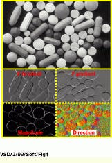
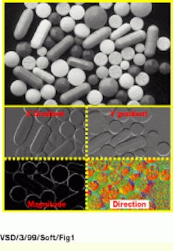
FIGURE 1. Mask-based edge operators usually produce a pair of output images. Applying a Sobel operator to the intensity image of the various pill sizes produces gradient magnitude and direction information (0 to 360 mapped onto colors from red through green to blue). Alternatively, the output can be viewed as separate x - difference (gradient) and y - difference (gradient) images, where brighter values correspond to positive changes, gray is no change, and darker colors represent negative changes in the gradient.
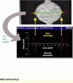
FIGURE 2. Gauging can be implemented by detecting sign changes (zero crossings) in the second derivative of a line profile across an object. The yellow cross hairs in the top image correspond to these crossings in the second derivative profile. Note that noise and local variations in the intensity cause many such crossings, but these can be filtered out based on criteria such as the slope of the crossing.
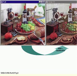
FIGURE 3. Edge-segmentation techniques are not limited to measurement and analysis applications, as illustrated by this cartooning of a scanned photograph. Once strong boundaries are detected with a difference-of-Gaussian function, they can be filled with new data such as the average color within each boundary.
ROBERT BELKNAP is director of software development, Imaging Products Division, Amerinex Applied Imaging Inc., Northampton, MA; [email protected].