What is deep learning and how do I deploy it in imaging?
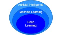
What is deep learning? Within the area of artificial intelligence (AI) exists machine learning, and within that, is the area of deep learning. Many different types of artificial intelligence exist. AI is any technique that imitates, at least in part, what a human would do with their mind. It is the ability of machines to mimic human behavior, and usually integrates perception, prediction, reasoning, and decision making, according to Yann LeCun, Vice President and Chief AI Scientist at Facebook.
Deep learning (Figure 1) can be thought of as “programming with data.” In a virtual machine setup with a neural network, the network is initially not programmed to do anything. When this virtual machine is given images, it begins to program itself to perform whatever the task is that is being set up. Deep learning can be used in imaging in many ways, including the recognition of objects in images, flaw detection, sorting and grading products, facial recognition, self-driving cars, and denoising images, among others.
Neural networks are modeled after the human brain. The brain consists of around 100 billion brain cells – neurons. Each neuron has dendrites (inputs), a nucleus, and axons (outputs). The connection between an axon of one neuron and a dendrite of another neuron is a synapse. The synapse contains a small gap separating the axon and dendrite, and when things are going right, there is dopamine in the synapse that strengthens the electrochemical connection the two neurons.
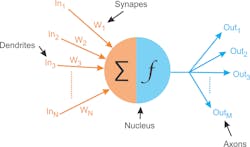
Something similar exists in a computer model of the neuron (Figure 2), with the nucleus and the dendrites (inputs) and the weights associated with each input, which represents the synapses—how tightly coupled the inputs are to preceding neurons. There are also the axons (outputs from the neurons). One important aspect of the computer simulation of a neuron is the activation function, which introduces non-linearity to neural networks. Activation functions include the sigmoid, hyperbolic tangent, rectified linear unit (ReLU), and leaky ReLU functions.
The simple neural network proposed many years ago consists of three layers. The input layer did nothing but distribute inputs and had no activation function or weights. Then there was the hidden layer in the middle, and the output layer. This was the minimal neural network architecture.
To use a neural network in deep learning, it must be trained to minimize errors over the training set. The training technique is backpropagation. When using the network, input data (images or features) advance through the neural network to reach the outputs. Network training involves starting from the output and propagating the error backwards through network (backpropagation). Network training uses the steepest gradient descent, which means using the derivative for the activation function and the chain rule in Calculus to move the errors back through the network regardless of the number of layers.
One learning control parameter, the learning rate, controls the magnitude of the weight adjustment based on the area and the steepness of the gradient. Starting with a very-high learning rate and trying to make big jumps in learning typically results in big weight changes causing the network to diverge from a solution and perform worse instead of better. When using a high learning rate, some learning takes place, but typically the network doesn’t improve to the point of being useful. Setting the learning rate low results in a long training period. A learning rate that brings the error down as quickly as possible is ideal, but ultimately, developers must experiment and configure the system to find the best learning rate.
In convolutional neural networks (CNN), an input (image), first goes into layers performing convolution with the convolution weights set through training. The next layers use an activation function, usually followed by a pooling layer, where groups of four pixels reduce to one, thus reducing the overall size of the image and making it easier for the network to extract features. Pooling can be 2 x 2 to 1, it can be 3 x 3 to 1, and it can be the maximum, the average, or the median, but the most common pooling function involves getting one pixel from the maximum of four pixels.
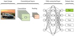
In the CNN, an image goes through a number of two-dimensional convolutional layers and then is flattened to create a one-dimensional feature vector from the image. The feature vector runs through additional network layers to create classification outputs (Figure 3). The next step involves non-maximum suppression, an important post-processing step. If the neural network says cat 0.8 and dog 0.3, and the application only requires choosing between cat or dog, non-maximum suppression helps determine that—based on the difference in values—a cat is in the image. An issue presents itself when the network says cat 0.51 and dog 0.49. Here, the non-maximum suppression algorithm must be strong enough to render such values as indeterminate.
Deep learning techniques and implementation
Techniques for using deep learning in imaging include supervised learning, the most common method, where a system trains with labeled images and is then tested. If the testing results are adequate, the deep learning-based system is ready to use. Transfer learning methods involve using supervised learning along with a pretrained neural network. In this method, retraining is only required on the later layers in the network for the new application. When it is appropriate, transfer learning is much faster than training a network from scratch.
Unsupervised learning, or predictive learning, defines classes based on clustering of input data without labeling. Reinforcement learning uses a reward—positive or negative—for each output during training. The learning rate is much slower than supervised learning and requires much more data. Lastly, adversarial training involves the use of two neural networks working against each other.
The first step in implementing deep learning into an imaging system involves determining the types and numbers of layers, the number of inputs (usually the number of pixels in the input images), and the number of outputs (usually dependent on the number of classes required). Inputs, images, outputs, and labels for the images then go into a model under training. Training compares the network’s outputs to the labels to generate an error signal which feeds back into the model under training to adjust the weights (coefficients), a process repeated until the error over all the training images reaches an acceptable minimum value.
When this happens, the network is tested using images not used for training to verify the network’s outputs have a sufficiently low error. After a successful test, this neural network can be exported with the trained weights and becomes the model to use. At runtime, the model loads into an inference engine—a computer running the neural network—where the trained network operates.
Deep learning requires an abundance of labeled training data. This data will be split up into three classes: training data, test data, and validation data. Training data is used exclusively for network training, with each pass through the training data representing an epoch. After each epoch, the network’s performance is evaluated using the validation data and the error on the validation data is tracked as an indication of how well training is progressing. After training—with the error on the training data sufficiently low—the network is tested using the test data to ensure acceptable results. Having a separate test set on which the network doesn’t train enables developers to independently test a trained network—providing the only evidence that a network performs reasonably well.
Several methods for speeding up training exist, such as initially training with a subset of the training data. Such a method helps get adequate weights. Another option, transfer learning, involves taking a CNN previously trained on a similar problem and only training the last few layers of the network for the new application. With a similar enough network, the features extract the same, removing the need to train the convolutional layers—it is only necessary to train the last few layers from the feature vector to output.
Fine tuning—another method similar to transfer learning to speed up training—involves using a new, small set of training images with a trained network. To use fine tuning, the output layer of the CNN must be replaced, with training performed with a small training data set. Pre-trained networks for transfer learning and fine tuning exist, including VGG-16, ResNet 50, DeepNet, and AlexNet by ImageNet.
Several considerations must be made when implementing a deep learning system, including the fact that a fast system requires parallel processing. A CPU can perform initial tests but will be very slow in training and execution. Useful tools for parallel processing include graphics processing units (GPU), field-programmable gate arrays (FPGA), and digital signal processors (DSP). Chips such as the Apple A12 bionic chip, which has two CPUs and a GPU, plus some additional circuitry specially designed to execute deep learning networks, as well as special processing chips like the Intel Movidius and Intel Nervana, also provide processing capabilities.
Data must also be considered, including data for training, validation and testing. More training data means better results. Implementing a successful deep learning system necessitates a lot of time and effort spent on gathering and labeling data.
Major challenges and pitfalls to avoid
One of the major challenges in deep learning involves real-time processing of many pixels, which means a lot of data, which requires a lot of computational power in both training and execution. This necessitates a very large set of pre-labeled, training images, but in some cases, labeled training datasets can be purchased. Another problem exists with the possibility of mislabeling of training data. Labeling just one image wrong results in degradation in performance of a trained neural network.
Bias in the training data represents another possible pitfall. More samples of one class than the other leads to difficulty in achieving good results on the classes with fewer examples. Data storage is another factor, including the image format and image storage options. When storing images on disks, it takes a long time for retrieval. Solid-state disks become preferable, but if there are a million RGB, megapixel images, storage requirements become enormous.
In using machine learning without deep learning, network inputs won’t be the images, but features extracted from the images. Selected features must be normalized in such scenarios. With one feature going from 0 to 1 and another feature that goes from 0 to 100, the latter dominates. Normalizing scales the features ensuring that they all fall within the same range. Otherwise, the network will fail to meet performance expectations.
Data augmentation—a method for reducing the cost of gathering and labeling the data—improves network reliability. Augmenting a picture of a cat by creating several other pictures from it with the same label represents one example. Further methods include rotation, scale, shear, obscuration (e.g. haze), color change, flip/mirror, crop, addition of noise, and varying of the background scene.
Choosing the right network configuration poses potential problems. If a network is too complex training time will be longer than necessary and the network may not generalize the features to recognize and actually perform poorly.
One option to deal with long training time is renting cloud processing time from Microsoft or Amazon for deploying deep learning applications, as the cloud pulls in many processors and GPUs to get training done more quickly. Determining the initial conditions of the network also creates a challenge, as does the selection of the learning rate and training parameters.
Pragmatic challenges in deep learning exist as well, including the input of an image during execution that is not representative of any training input (an anomaly). Security must also be considered, in terms of what would happen when a network fails to give the right answer or if someone hacks into the network.
Philosophical challenges must be considered as well. CNNs lack creativity or abstract thinking, have no intuition, and cannot synthesize input from a specified output, unlike people. For example, it is not possible to tell a network “I want to recognize a cat, what do I look for?” Other questions to consider are: If the network fails, who is responsible, and will they be able to explain why?
Supervised learning and reinforcement learning are not sufficient for real world problems. Unsupervised learning is required, where the network can not only recognize the cat and the dog, but also look at a picture of a camel and determine that it is not a cat and not a dog.
Several methods for improving efficiency in deep learning exist, including experimentation with floating point weights and subsequent reduction to integer (fixed point) weights, which leads to speed increases but a slight decrease in accuracy. Using binary weights (0 or 1) also leads to a further increase in speed, but a decrease in accuracy.
In a network with lots of branches with weights, some of these weights become infinitesimally small. Pruning these weights out is possible, with only a small decrease in accuracy. Transfer learning can also lead to a significant reduction in training time.
Tips for successful implementation
Regarding the successful implementation of a deep learning system, here are several tips to consider. First, watch out for overfitting, which happens when a neural network essentially “memorizes” the training data. Overfitting results in great performance on training data, but the network’s model becomes useless for out-of-sample prediction. Larger networks are more powerful, but it becomes easier to overfit. A system trying to learn a million parameters from 10,000 examples is not ideal. If parameters are greater than examples, this leads to trouble. More data is almost always better because it helps fight overfitting.
Validation—and one should never train on the validation or test data—really helps when the network isn’t behaving right, and validation doesn’t track the testing results. When this happens, stop and make changes to the network rather than continuing with disappointing results.
Furthermore, train over multiple epochs. With learning rates of 1/10th or 1/20th, many passes are required to get the gradient down to the minimum or near the minimum. Lastly, stacking layers can help as well. The first layer can be a convolutional layer or multiple convolutional layers doing different things.
When approached with great attention to detail and an understanding of deep learning architectures, functionality, and system requirements, the technology offers great enhancements in efficiency and accuracy in machine vision processes of all kinds. Additionally, in the coming year, breakthroughs should be coming, in network topology, in ways to speed up training, in ways to reduce the number of labeled images needed to train, and even in new types of networks for learning, which will only have a positive impact on the machine vision community.
Perry West is the founder and president of Automated Vision Systems, Inc. (San Jose, CA, USA; www.autovis.com)
About the Author

Perry West
Founder and President
Perry C. West is founder and president of Automated Vision Systems, Inc., a leading consulting firm in the field of machine vision. His machine vision experience spans more than 30 years and includes system design and development, software development of both general purpose and application specific software packages, optical engineering for both lighting and imaging, camera and interface design, education and training, manufacturing management, engineering management, and marketing studies. He earned his BSEE at the University of California at Berkeley, and is a past President of the Machine Vision Association of SME Among his awards are the MVA/SME Chairman’s Award for 1990, and the 2003 Automated Imaging Association’s annual Achievement Award.