Fundamentals of Optics - An Introduction for Beginners
What Is Optics? Introduction to Optics
*By Reinhard Jenny,Volpi AG
*Translated By Scott Kittelberger,Volpi AG
1.0 Historical Overview
The ability of Man, and various animals groups, to visually perceive their surroundings is realized by the eye and coupled nerve endings in the brain. To describe this ability, the Greeks used the word "optikos," which can be interpreted as seeing, vision, or visual faculty.
The origins and historical development of our current knowledge of optics are very interesting. Archaeological findings from the time of the Pharaohs (2600-2400BC) have shown this culture possessed outstanding anatomical knowledge. It is known that when observing a statue, it appears the statue is always looking at you, even when you are in motion. Precise studies have shown that the ingenious combination of a plano convex lens with a properly positioned pupil and a short focal length concave surface are responsible for this effect.
Discoveries dated to the 11th and 12th centuries A.D. on the island of Gotland, Sweden (once populated by Vikings) produced aspherical lenses. These lenses can be compared with those produced today by modern methods and the advice of scientists. At many different periods it was known that optimized lens surfaces produce better image quality. These lenses were most likely used to cauterize wounds, ignite fires or as loupes for handworkers.
Leonardo da Vinci (1452-1519) in one of his many discoveries used a lens to project light from a light source. He described optics as a "Paradise for Mathematicians" and meant principally to give a new perspective to the topic of geometrical optics.
The scientific development of optics, specifically geometrical optics, evolved from the contributions of many. Fundamental work in diffraction by Snellius (1591-1626), in addition to the insights and refinements of Descartes (1596-1650), led to the demonstration of a rainbow, on the basis of the fundamental laws of refraction. Galileo Galilei (1564-1642) made further contributions with his researches into telescopes and observations of the moons of Jupiter in1610.
Shortly afterwards, Huygens (1629-1695) reached his description of double refraction in calcite (Traité de la Lumière, 1690) with the help of his assumption that the plane of light wave oscillation can be chosen with respect to the optical axis of the calcite crystal. He has been recognized since that time as the founder of wave theory. Isaac Newton (1643-1727), aside from his studies of gravitation, worked on the origins of white light and color on glass plates (Interference of Light). Trained as a glass blower and binocular maker, Fraunhofer (1787-1826) constructed the first grating structure. Light is diffracted into its spectral components. He assembled the first spectroscope and studied the spectrum of sunlight (Fraunhofer Lines). He is known as the father of spectroscopy and astrophysics. Fresnel (1788-1827) furthered wave theory and developed the formalism of light reflection, i.e., dependence of transmission on the angle of incidence.
The demonstration of the magnetic field components of light, by Faraday, in 1845 led Maxwell to formulate the general consistency of the propagation of light as electromagnetic waves. The famous "Maxwell Equations" were described in his "Treatise" of 1873. Max Planck (1858-1947) in 1900, presented his results of the quantum nature of light (light can be divided up into small quantities of energy). In 1905 A. Einstein broadened our understanding of light to include the quantum and particle nature of light with the concept of photons.
Further considerations of this new quantum theory led to the development of Quantum Mechanics with many new realizations and results in physical optics (Quantum Optics). Some examples are:
1887: H. Hertz (1857-1894) => Photoelectric Effect
1917: A. Einstein => stimulated emission => require for lasers
1960: T. Maiman => first laser (Ruby) developed
1949: Bardeen => first transistor
1960: Light emitting diodes (GaAs based)
1960: Development of "Non-Linear" Optics
Effects in liquids, gases. and mostly solids where: the frequency of light may be doubled, self focusing of light, reversal of wave fronts (phase conjugation), variation in the index of refraction with light intensity (photorefractive effect), and many other effects which were the direct result of high intensity laser beams.
1970: Work in integrated optics dealing with the coupling of and the guiding of light in microscopic structures (thin films, glass fibers, dot structures in crystals, etc.) These were the basis for optical switches for use in future computers.
These summarized scientific discoveries describe wave optics and geometrical optics (which is a special case of wave optics), on the one hand. On the other hand, the innovative results of quantum optics have strongly influenced the scientific world.
For completeness, other areas of optics should be mentioned, namely that of Helmholz (1821-1894) described as "physiological optics." Here, underlying laws of our mind and psyche are considered that are not part of the physical theory. As we are interested in geometrical optics, we have established this to be but a part of the whole of optics. We will mainly deal with insights into the workings of optical systems.
2.0 Propagation Characteristics of Light
2.1 The Wave Nature of Light
Electromagnetic waves are described by electric and magnetic field components. They travel in the form of a wave. A wavelength can be associated with these fields. A relatively small part of the electromagnetic spectrum is physiologically detected as color by our eye. We commonly describe this part of the spectrum as light. The spectrum spans shorter wavelengths such as ultraviolet, x-rays, and gamma rays. Longer wavelengths span the infrared, and on into those larger than 1mm, microwaves (telecommunication, radio , television, etc.).
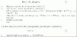
Electric and magnetic field components can be physically measured. The height (amplitude) of the wave varies with time. If we were to observe the wavelike propagation of the electric field E(x,t), we would find it can be mathematically described as:

null
The expression in parenthesis on the right hand side of Equation (1), which will be referred to as the argument, should be noted. The first term, wt, is the time component and the second, kx, the spatial component of propagation.
The following example shows the effect these components have on wave propagation.
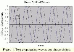
Figure 1 shows two independent waves propagating. At t=0, one wave has an electric field strength, E1=0, while the other, E2, has a non-zero amplitude. At time t=0, the argument of the sine function in (1) becomes kx. We therefore have E1 (x,0) = 0. This means the product, kx, must equal Npi, (where N = 0,±1,±2,....). E2 has a negative amplitude at t=0, suggesting that kx is not a multiple of pi. In this case we refer to the E2 wave as being "phase shifted" from E1.
The condition of this shift in position between the two waves will not change as the waves propagate further in space, so long as the waves are undisturbed. The contribution of kx describes the spatial phase of a wave at position x.
2.2 Interference
If two or more waves meet at a point x, the contribution and position of the field components, E1 and E2, can be superimposed on each other. Superposition (± Interference) does not take place if the field amplitudes are oriented perpendicular to each other.
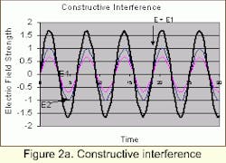
Figure 2 shows the superposition of two sine waves. The respective amplitudes and phases differ from each other. Comparing the resultant field amplitude, E, with the individual components, E1 and E2, we observe in Figure 2a an increase in amplitude. This is constructive interference: the phase difference between E1 and E2 is zero or multiples of 2p. (Dj =N · 2pi , N = 0, +1, +2,.... ) Destructive interference is shown in Figure 2b where there is a decrease in the resultant field amplitude. The phase difference between the two waves is half of one wavelength (Dj =(2N+1) · pi). If the constituent amplitudes would have the same amplitude and differ in phase by half a wavelength (Dj =(2N+1) · pi), the resultant amplitude would be zero.
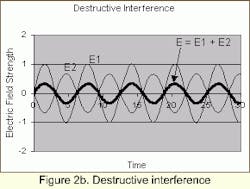
Superposition of a constructive nature leads to an increase in light intensity (high intensity), whereas destructive interference leads to a decrease in intensity or even zero intensity. This effect can be seen in the case of two beams propagating in different directions, which simultaneously impinge on a screen at the same coordinate. One can observe the periodic pattern of light and dark stripes (double slit interference). This pattern will appear everywhere the two beams superimpose.
The ability of light to interfere, along with the observations of von Huygens that wavefronts themselves can become wave centers of point source propagation, explains the effect of diffraction.
2.3 Diffraction
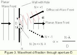
A plane wave impinging on a geometric structure with an opening (wall with a round opening = aperture) will emit elementary point source waves from each opening. The projected pattern of these waves oscillates between bright and dark areas, which are not sharply separated. This oscillatory transition is the result of interference of these elementary waves. The phase difference between neighboring maxima or minima is always 2pi.
Diffraction therefore means that wave fronts traveling in a straight line, which are then restricted by some opening, divert off their straight path into light/dark patterns. This assumes, of course, that the waves don't experience other phenomena such as reflection or refraction. In Figure 3, one can see deviation of the diffracted light from the original angle impinging the wall. The optical path difference, (N·lambda), between rays emanating from the edges of the opening and the size of the geometrical opening, D, will determine the Nth order diffraction angle.
null
Each N = ±1, ±2, defines a direction a, or for small angles, Na, of an intensity maximum. The intensity pattern at the edges due to contributions from non-diffracted rays leads to a reduced sharpness of bright/dark transition. We refer to this as reduced contrast.
The direction of rays and therefore of diffracted rays rays is always perpendicular to their wave surface.
Geometrical optics neglects diffraction in progressive ray calculations. One assumes = 0 to be a boundary condition of wave optics. All cross rays in the system have a diffraction
2.3 Refraction
Aside from propagating in air or in a vacuum, there are other media (liquid, gas, and solid) in which light can propagate. We differentiate between optically transparent (dielectric) and absorbing media. Due to different material characteristics, such as chemical composition and consequent atomic characteristics, light propagating through a medium will interact with the electrons in the outermost shell. The effect is to redirect the light and alter its speed of propagation. This and other effects are linked to the index of refraction.
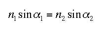
With increased number of electrons influenced by the electromagnetic field, and increased frequency (reduced wavelength), the index of refraction of the material generally increases. The index of refraction is wavelength or frequency dependent (dispersion). If light of a given wavelength impinges the interface of two media at an angle (assuming different indices of refraction), there is a change in direction in the given by the Law of Refraction:
null
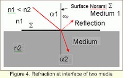
where n1, n2 are indices of refraction of the media 1 and 2, respectively, and a1 and a2 are the angle of incidence and angle of refraction, respectively. Light moving from an optically less dense material to optically more dense material will be refracted toward the surface normal (Fig. 4). In the opposite case, the light will be refracted away from the normal.
As can be seen in Figure 4, when refraction occurs, a portion of the light is also reflected. The reflected beam exists in a medium with the same index of refraction as the incident beam. This is described by the Law of Reflection.

null
The negative sign in Equation (4) indicates a reversal of direction for the reflected beam.
As described above, refraction is related to the differing speed of light in various media. The Law of Refraction can also be stated as:
null
Take, as an example, air to be medium 1. The index of refraction of air is nearly n1 = 1 and the corresponding speed of light is approximately that of vacuum. In accordance with Equation (5), the propagating speed of light in medium 2 is:
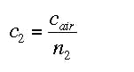
null
Equation (6) infers that the speed of light in an optical medium more dense than air is smaller than air. Only in a vacuum or in a medium less dense than that of air is speed of light greater than in air.
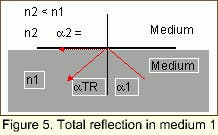
As is known trigonometrically, the sine function has a maximum value of 1. The Law of Refraction suggests that light passes from one media to the next. It follows that angles of refraction larger than 90° does not result in refraction, but rather in total reflection in the optically denser material.
The limiting angle for total reflection from medium 1 to air as medium 2 yields the following expression of the Law of Refraction:
null
Total reflection is a prerequisite for guided waves in optical fibers and light guides. The optically denser material is the core (usually glass, quartz, or plastic) and the cladding is an optically less dense material of glass, quartz, or plastic. The specific selection of core and cladding materials will result in a specific numerical aperture or acceptance angle for the fiber
3. Optical Image Formation and Optical Systems
Certainly, the concept of optical phenomena was first realized from observing nature, i.e., rainbows, light beams redirecting, color effects of light shining through crystals, and refraction on water surfaces. In an effort to reproduce these effects, attempts were made to construct experiments, which could use these effects. The scientific approach was also employed, which made use of the many observations. Formulating laws was attempted through sketching diagrams and experimentally varying parameters. For more than 1000 years the Law of Refraction was not known in its current mathematical form, in spite of the fact that there are clear indications that people knew how to work with transparent crystals and aided vision with enlarging optics. The predecessor of today's geometrical optics was the telescope builder of the 16th and 17th century, above all Galileo Galilei. They searched for homogeneous materials without inclusions or spatial variations in the index of refraction. Attention was given to work methods, which yielded good surface quality and polishes, so as not to affect image formation by way of scattering effects. (It is noteworthy that Fresnel experimented with various natural crystals. A type of lens, the Fresnel lens, with many ground prismatic rings was named after him).
3.1 Optical Image Formation
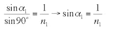
In optical image formation, we understand a point source of light to be placed at an object point. This point propagates by way of a diverging image bundle (homocentric bundle) through an optical system to a corresponding point in the image plane (image point). At this point the rays from the point source converge again (Fig. 6). A particularly good image results when all rays within a region (i.e., lambda/4) interfere constructively. If the image lies behind the optical system, where the emitted object rays define the direction, the image is called a real image. If the image lies in front of the optical system, the image is called a virtual image.
A virtual image can not be acquired by any sensor behind the optical system without additional optical elements. Sensors can only acquire real images.
In Figure 6, the constructed ray which creates O' obviously doesn't exist at infinity. The lens in our eye can, however, focus divergent rays from a virtual image onto the retina and simulate the existence of a virtual image at point O'.
3.1 Optical Elements
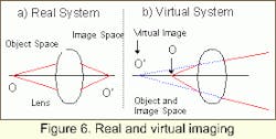
In technical optics, image formation is achieved with lensing systems integrated with optical elements, which alter light, such as prisms and mirrors. Lenses are transparent elements (for spectrums of interest) made usually of glass. The entrance and exiting surfaces are usually spherically ground and polished. We differentiate between converging lenses with positive refractive power and diverging lenses with negative refractive power.
Parallel rays falling on a converging lens will be refracted to the focal point located behind the lens. The same experiment performed on a divergent lens will disperse light. Rays will not converge behind the lens, but will yield the projection of a virtual image point in the object space.
Lens Types
The following lens types are used for conventional optical systems.
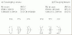
null
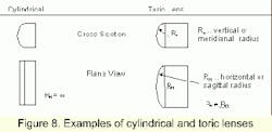
Rotationally symmetric lenses are generally used for optical systems, meaning that the refractive surfaces are spherical or conical and a useful outer diameter is concentrically ground. Some non-rotationally symmetric lenses are, for example, cylindrical or toric lenses. These lenses have differing vertical and horizontal cross sections.
Currently, more and more compact video camera systems are using rotationally symmetric aspherical lens systems. Imaging errors can be reduced which occur mainly from slight conical form (spherical aberrations) of spherical lenses (Fig. 9).
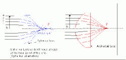
null
Figure 9. Difference between focusing ability of spherical and aspherical lenses
4.0 Basic Design Concepts of Optical Systems
4.1 Designations and Conventions
Using a real image formation system with a single lens (single step system), we would like to know the important parameters that describe such a system. The lens is placed a certain distance from the object (Object distance a). The direction of propagation is defined from the object to lens for this system. The region before the lens is referred to as the object space. In the even of a real image, the image space lies behind the lens. The distance between the lens and the image is referred to as the image distance a'.
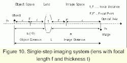
Figure 10 has sufficient parameters to calculate the most important dimensional quantities of an imaging system, such as linear magnification, acceptance angle, and field of view (FOV). The convention of a negative symbol (-), such as a negative object distance (a < 0), is relevant here. If a virtual image lies in the object space, a' negative is inserted.
The following expressions are valid, to first order, for rays whose angle are small relative to the optical axis [a = sin (a)]. These are called paraxial rays. One of the most important equations characterizing optical imaging is the conjugate distance equation. For a given lens of focal length f, the expression relates the object and image distance.
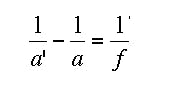
null
This expression is based on the assumption that the lens thickness t is small relative to a and a', so that the lens is considered thin. Consequently, one can conclude that the sum of a (notice the negative) and a' yields the object-image distance, L (t=0).
null
The linear magnification is define by the ratio of image/object distance
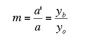
null
The relationship of the distance yb/yo (Fig. 10) is the actual linear magnification. This may deviate from expected magnification due to effects such as magnification distortion or deviations from paraxial assumptions. For small angles of FOV, both quotients should be identical. The actual image of an object through single converging lens has a negative magnification (m < 0) resulting from the negative object distance (a < 0). For a virtual image, m is positive (a < 0; a' < 0). A negative magnification implies the image is inverted from that of the object (upside-down image).
By combining Equations (8), (9) and (10), the following useful relationships apply to paraxial systems:
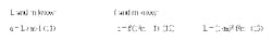
null
Paraxial systems with thin lenses are a simplified configuration for crudely analyzing optical systems. They present a special case. Realistic systems use thick lenses and relatively large acceptance angles [alpha ¬ sin (alpha)], so that the paraxial assumption needs to be extended.
Thick lenses have two refracting surfaces to which the thin lens parameters can be applied. They are referred to as principle planes (object side h, image side h'). The corresponding intersection points with the optical axes are principle or nodal points (H and H'). Equation 8 is used by replacing object and image distances with nodal points.
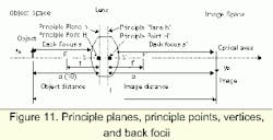
Using zz' = -f2 (Fig. 10), the imaging formulae can be expressed with reference to the focal points. Here, z and z' are the distance to the object and image from their respective focal points.
In general, the object principle plane is nearer the object than the image principle plane, but this can be reversed with thick lenses and unique surface configurations.
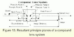
The intersection of the polished lens surface with the optical axes is called the object vertex, S, and the image vertex, S'. The corresponding distances between vertex and object or image are referred to as the back focus, s and s'. Optical systems usually contain converging and diverging lenses made of different materials. Such systems are known as compound lens systems. A compound lens system can also produce an object and image principle plane. The intersection of the outer most lens surface with the optical axes defines the vertex and associated back focus.
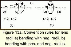
Lenses in an optical system can have different shapes or bends with radii r1 and r2. Note that for most compound systems (rotationally symmetric), the center point of all refractive surfaces lies on the optical axes. If the radius is to the left of the lens (toward the object), it is negative by convention and to the right of the lens it is positive. By way of this lens bending, the location of the principle plane can be influenced.
The following expressions are important characterization of lenses in air:
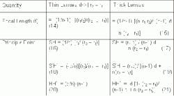
null
Lens Equation for thick and thin lenses (d..Lens thickness; n...index of refraction of glass)
Note for infinitely thin lenses (d=0), with focal length according to (14), implies SH=S'H'=HH'=0 (16)-(21). The lens collapses to a single principle plane.
It is possible for the image side principle plane, H', to be closer to the object than the corresponding object side principle plane, H (HH'< 0). This is for case where d > (r1 - r2).
Figure 14. In choosing a meniscus lens (b), as opposed to a symmetrical lens (a), the object related back focus can be shortened, thus maintaining the same focal length. (Examples: condensor, lenses, telescopic systems, etc.)
For understanding optical configurations and instruments, the choice of the principle plane location is an important characteristic. For example, large focal length lenses with short back foci can be conceptualized.
The arrangement of several single lens systems into a compound lens system will combine the different bendings, glasses, thicknesses of individual lenses, and lens distances into a single system. A single object side and image side principle plane describe such a system.
4.2 Lensing System Apertures
The aperture of a lens system is understood to be the relationship between the system focal length and the free diameter of the system. This is especially true of systems whose object or image back focus is infinite. This is usually true of photographic lenses where the object is at infinity and the image side back focus is very short.
The aperture number is given by:
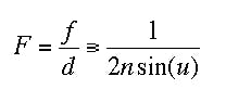
null
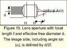
The included angle between the outermost ray and the optical axis is related to the aperture of a lens. One can easily see from Equation (22) that d = 2 f n sin (u) (n.. index of refraction).
According to Equation (22), systems with large aperture have small aperture numbers. The aperture numbers of most lenses are assigned a number according to the diaphragm range. This range is defined such that a step in aperture number reflects a factor of 2 change in the light flux. The diaphragm range is as follows:
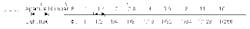
null
The relationship between relative light flux and aperture number is:
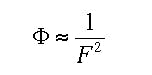
null
Optical professionals sometimes refer to the numerical aperture of a lens system. This is defined as:
null
where the index of refraction is that of the medium where u appears. From Equation (22) the relationship between numerical aperture and aperture number can be readily seen.
null
Systems with infinitely large back foci (or object distances) exhibit infinitely small magnification (m = 0). See Equation (10). Frequently, lens systems project an object onto an image sensor in the image space that is made of photosensitive material. Most magnification ranges between -10 < m < 0.
If one concretely wants to know the effective aperture number, Feff, of an imaging system (magnification m ), it can be derived from Equations (8), (10), and (22):
null
Feff..effective aperture number, F·...aperture number m = 0, m...magnification (m < 0)
Equation (26) shows, that for magnification m < 0, the effective aperture number is always larger than that of a system with magnification m = 0. According to Equation (25), it is also evident that the corresponding effective aperture is always smaller than that when m = 0.
4.3 Irises and Pupils
Optical systems are often designed with a fixed or variable iris. For single lens systems, the lens diameter can act as the iris at the principle plane. Irises, also called aperture stops, are precise mechanical apertures, which restrict light rays transmitted through a lens. This restricting is obviously related to the aperture number. The free diameter in Equation (22) can be replaced with the aperture diameter. The iris defines the amount of light flux transmitted by an optical system.
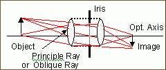
Figure 16 schematically shows the rays transmitted through an optical system with an iris. Typically, the middle ray of a ray bundle (principle ray) intersects the optical axis at the iris plane. The corresponding peripheral ray is restricted by the iris.
Depending on the lens system, the position of the iris may be in the middle of system or shifted in front of, or behind, the precise center. In general, by shifting the location of the iris, the oblique aberrations of a lens system (such as coma, astigmatism, distortion, lateral color) can be influenced and minimized.
A lens stack will, in most cases, create a virtual image of the iris in image planes in front of, and behind the iris. The iris image appears as a typical limiting ray diameter when viewing the lens. These iris images are also called pupils. The front and back images of the iris are called entrance pupil (EP) and exit pupil (XP), respectively.
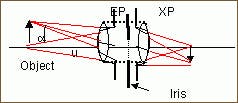
Figure 17 is a schematic diagram of the pupils. Ray bundles emitted from the object or in the reverse direction from the image are restricted by their respective pupils, and their propagation direction is defined.
4.4 Light Energy Collection of Optical Systems
The size of the entrance pupil and therefore the size of the aperture are definitive for the transmitted luminous flux. The magnitude is given by the following expression

null
B....luminance (lumen/sr/cm2)
F....illuminated area (cm2) of the Object
u....half angle of the emitted beam (Fig. 17)
Equation (26) is only valid for the imaging of light emitting points lying on the optical axis. When the luminous flux of light emitting points transmitted through optics is not lying on the optical axis, then the optical axis is smaller than Equation (26).
Equation (26) is reduced by a factor cos4(alpha), thereby formulating the cos4 - Law for off-axis points
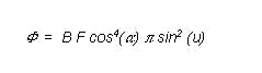
null
alpha ... angle between the main ray and the optical axis.
4.5 Depth of Field of Optical Systems
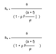
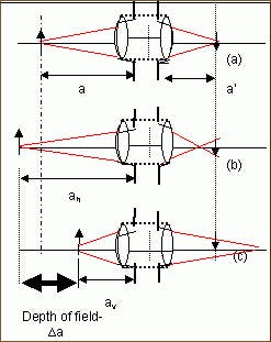
The aperture of an optical system will set the sharpness region of imaging, given at various object distances. The sharpness region increases as the aperture number decreases. For object distance a, focal length f, and aperture number F, the limits of the object distance av and ah are related by
null
a ... Object distance for theoretically sharp imaging (Fig. 18)
f ... Lens focal length; F ... Aperture number; p ... Circle of confusion diameter
Here, av and ah are the shortest and longest distance locations which can be sharply imaged by:
null
The permissible circle of confusion diameter, p, for an image point refers to the dimension of the image, being approximately one thousandth of the image diagonal.

null
The depth of field, ah - av, is calculated by subtracting Equation (28) from Equation (29), and also using Equation (12).
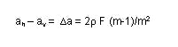
null
It can be seen from Equation (31) the depth of field can be increased by choosing larger aperture numbers (smaller apertures), and smaller magnifications.
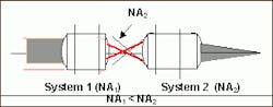
4.6 Numerical Aperture Interface Requirements
Should several optical systems be assembled in series, each individual apertures of each system must be paid attention to for optimal energy transmission. As a basic theoretical requirement, two optical systems must have matched numerical apertures at their point of coupling.
null
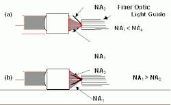
The same requirements hold for coupling light in and out of fiber optic light guides.
null
Figure 20. Optical lenses for coupling to glass fibers a) NA1 < NA2 and
b) NA1 > NA2
Several things can jeopardize light transport through fibers. If the coupling light has a smaller aperture than the fiber (Figure 20a), one would want to maintain the coupled luminous flux over the whole length of the fiber. The light transmission will remain more constant for applications where the fiber moves (varying bend radius) than with an impinging beam of larger aperture than that of the fiber (Figure 20b). An under filled numerical aperture is therefore desired for measurement applications.
4.7 Telecentric Lenses
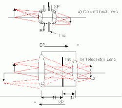
Another important configuration issue for measurement systems is the pupil location of telecentric optics. With conventional projection lenses, the pupil plane is usually located within the lens. The entrance pupil of a telecentric system is at an infinite distance in front of the first lens plane and therefore the object.
Entrance - and Exit Pupils of a fully telecentric lens (or both sides of a telecentric lens) are at infinite distance from the corresponding object - or image locations.
null
Figure 21. Beam patterns of a conventional lens a) and a telecentric lens b)
Due to the excellent position of the iris, distance f1 from L1, the corresponding aperture image (entrance pupil) is an infinite distance from the object. The principle rays are therefore parallel to the optical axis. In other words, the principal rays from all object points are effectively parallel rays, all displaying similar projection characteristics.
Often, the rays are oriented such that the principle rays are parallel to the optical axis in the image space. This compound lens configuration shows the unusual feature that the total focal length is infinite. For the total focal length of a compound lens system
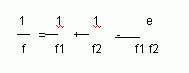
null
e = distance between lenses ; f1, f2 = Focal length of lens L1 and L2; f = Total focal length
For a telecentric lenses, e = f1+f2. Equation (33) yields: f = ∞.
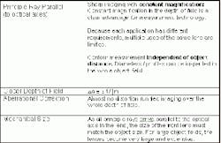
These characteristics differentiate telecentric and conventional optical systems
null
*Reinhard Jenny
M.S. Physics, Technical University Graz (Austria)
Vice President for Research and Development
*Scott Kittelberger
M.S Physics, Syracuse University (USA)
Volpi AG
Wiesenstrasse 33
CH 8952 Schlieren, Switzerland
www.volpi.ch
Volpi Manufacturing USA Co. Inc.R5 Commerce Way
Auburn, NY 13210 USA
www.volpiusa.com