Filtering techniques eliminate Gaussian image noise

Gaussian Filter Techniques Remove Noise From Image

Noisy images create problems in machine vision applications. Spatial filtering methods for removing noise have existed for more than a decade, but face problems like over smoothing without any preservation of edges, gradient reversal artifacts, ringing artifacts, and shift variance.

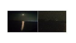
For machine vision and imaging tasks, step one in finding eventual success is getting the highly informative image.  Many types of noise exist, including salt and pepper noise, impulse noise, and speckle noise, but Gaussian noise is the most common type found in digital imaging. Within digital imaging, Gaussian noise occurs as a result of sensor limitations during image acquisition under low-light conditions, which make it difficult for the visible light sensors to efficiently capture details of the scene.

Mathematically, Gaussian noise can be characterized by the equation of the bivariate circular Gaussian function as:

Where, σx and σy represents standard deviations, μx and μy the means. The standard deviation shows the dispersion from the mean. Graphically, the variation in function value with variation in value of standard deviation is shown in Figure 2. Not only does the maximum value of the function decrease with increasing sigma, but the variation of other values from the mean or the expected value also increases [4].

Newer filtering methods like block-matching and 3D filtering (BM3D), non-linear means (NLM) filtering, and Shearlet transform prove more effective than previous methods used to remove noise. Spatial filtering techniques modify the spatial features of an image. A spatial filtering kernel helps facilitate spatial filter implementation.  Convolution of a smoothing kernel with the desired noisy images produces a denoised image. Based on the property of these kernels, different denoising results can be obtained. For example, a Gaussian kernel is obtained by plugging in different space values for x and y into the equation (1), and by controlling the value of sigma, the degree of smoothing can also be controlled.

Uniform image smoothing represents the main problem encountered with primitive filters, as doing so results in compromised important details [8]. Introducing range parameters into the Gaussian equation helps avoid the smoothing operation at the edges and contours and thus solve the problem. Using this filter—a bilateral filter [9]—introduces artifacts into the resulting image, however. A guided filter offers a more effective, edge aware spatial filtering approach. This filter uses a guidance image to effectively smooth consistent pixel intensity areas while retaining important detail information with the help of a guidance image. This filter is effective in removing artifacts [10]. Another filter effective in removing artifacts while preserving semantically meaningful information is the anisotropic diffusion filter, which uses second order partial differential equations with necessary parametric variations for smoothing [7].

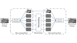
On the other hand, transforms use orthonormal filter banks to decompose images into low frequency and high frequency sub-band images. The low-frequency information contains the uniform pixel intensity areas and high frequency information contains all the edges and contours present in the image. A transform is considered effective in separating information if it can extract edges and contours out of multiple directions in the image. For example, a wavelet transform extracts high frequency information in three directions—horizontal, vertical, and diagonal—whereas the shearlet transform extracts information in multiple directions.

Gaussian noise affects higher frequencies. Applying a thresholding operation to high frequency (detail) sub-bands eliminates noise. As transforming an image takes it into another domain, coefficients are obtained as a result. To retrieve original pixel intensities, inverse transform applies to these modified coefficients, a process that lays down the complete picture of denoising more comprehensively because of its information separation strategy [2], [11].

NLM filtering, weighted least square (WLS) filter, and BM3D filtering represent more sophisticated strategies for achieving better results. In WLS filtering, the weighted least square energy function is minimized to obtain the output, so in this strategy, recursive filtering applies to the noisy image. This filter is fast and effective in removing halo artifacts [13]. NLM filters prove more effective in removing the outliers and mainly, shot noise. The nonlinearity of these filters helps to effectively remove the background noise while preserving meaningful information [8].

BM3D algorithms group fragments of images based on their similarity (block matching) and filter every fragment [12]. The BM3D approach is a very effective approach, with the smallest computational load.

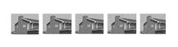
For experimentation, a mobile device camera with dual camera setup with 12 MPixel camera sensor and 13 MPixel depth sensor for emphasizing objects in a scene provides images. Images in Figure 5 show the results of a standard image of a house contaminated by Gaussian noise of different standard deviation (sigma). In this experiment, images with Gaussian noise with sigma 30 are used. When higher sigma noise is added, the image gets more distorted and more difficult to recover. 

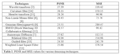
For testing, the two most popular and widely used metrics evaluate the performance: peak signal-to-noise ratio (PSNR) and mean square error (MSE): The two metrics can be explained as follows:

The higher the MSE value, the lower the denoised image quality. Hence, lower value of MSE indicates good denoising technique performance.

b) PSNR: Measure of signal power compared to noise power. The higher the ratio, the higher the visual quality of the image. Mathematically it can be written as [5]:

Here, L=255 and MSE is the mean square error.

Table 1 shows the values of PSNR and MSE for various denoising techniques. The metrics values can be compared with the visual results of various denoising techniques (Figure 6). Some state-of-the-art techniques like block-matching and 3D filtering (BM3D), non-linear means filter, and Shearlet transform perform best among all techniques.

Used for the experiments is an Intel Core (TM) i5-72000U- CPU @2.50Ghz processor and 8 Gb memory using MATLAB software. To start, Gaussian noise is applied to a 256 x 256 clean image. The filters and transform domain methods remove the noise from the images, while preserving the edges and details. Performance decreases as the variance of the noise increases. The new methods are primarily representative of the improvement of primitive spatial filters and transforms.

When compared to the original image, the visual results tend to lose some details, but the freedom of choosing parameters for the degree or smooth provides flexibility for using these techniques in disparate applications.

Several spatial filtering techniques can remove Gaussian noise. Additionally, some transform techniques can also remove noise from images. Spatial filters do not break the image into its high and low frequency components but apply directly to an image to modify pixels spatially to remove the noise (Figure 3). Transforms first break an image into scales of low and high frequency information (multi-scale decomposition, or MSD) then a thresholding operation applies to various components and an inverse transform applies to recover a noise-free image (Figure 4).

Noise impacts the higher frequencies of an image, so the thresholding operation only applies to the high-frequency layers. All spatial filters employed to remove noise remove higher frequencies present in the image. As the important edge and contour information is also high frequency information, a spatial filter or transform must remove noise without affecting the relevant edges and contours. All spatial filters or transforms proposed through the years have tried to solve this problem [3], [4], [5], but block matching and 3D filtering (BM3D), non-linear means filter, and Shearlet transform perform best.

Ayush Dogra is CSIR-Nehru Postdoctoral Fellow at CSIR-CSIO (Chandigarh, India; www.csio.res.in); Bhawna Goyal is Assistant Professor in the Department of Electronics and Communications at Chandigarh University (Punjab, India; www.cuchd.in); Sunil Agrawal and Renu Vig are professors in the Department of Electronics and Communication at UIET, Panjab University (Chandigarh, India; www.puchd.ac.in) and Apoorav Maulik Sharma is a research scholar at UIET, Panjab University.

References:

1.      Russo, F., A method for estimation and filtering of Gaussian noise in images. IEEE Trans. Instrum. Meas. 52(4):1148–1154, 2003.

2.       Vermaa A. and Shrey A., Image Denoising in Wavelet Domain, 1–10.

3.       Sairam, R. M., Sharma, S., and Gupta, K., Study of Denoising Method of Images-A Review. Journal of Engineering Science and Technology Review 8(5):41–48, 2013.

4.       Gonzalez, R. C., and Richard, E. W., Image processing. Digital image processing 2, 2007.

5.       Goyal, B., Dogra, A., Agrawal, S., Sohi, B. S., & Sharma, A. (2020). Image denoising review: From classical to state-of-the-art approaches. Information Fusion, 55, 220-244.

6.       L. Shapiro, G. Linda, Stockman, Computer Vision, Prentice-Hall, 2001.

7.       P. Perona, J. Malik, Scale-space and edge detection using anisotropic diffusion, IEEE Trans. Pattern Anal. Mach. Intell. 12 (7) (1990) 629–639.

8.       L. Shao, R. Yan, X. Li, Y. Liu, From heuristic optimization to dictionary learning: a review and comprehensive comparison of image denoising algorithms, IEEE Trans. 
Cybern. 44 (7) (2014) 1001–1013. 


9.       C. Tomasi, R. Manduchi, Bilateral filtering for gray and color images, in: Computer 
Vision, 1998. Sixth International Conference on, 1998, pp. 839–846.

10.    K. He, J. Sun, X. Tang, Guided image filtering, in: European Conference on Computer Vision, 2010, pp. 1–14. 


11.    transform, Appl. Comput. Harmon. Anal. 25 (1) (2008) 25–46.

12.    K. Dabov, A. Foi, V. Katkovnik, K. Egiazarian, Image denoising by sparse 3-D transform-domain collaborative filtering, IEEE Trans. Image Process. 16 (8) (2007) 2080–2095.

13.    Rahman, M. A., Dash, P. K., &Downton, E. R. (1982). Digital protection of power transformer based on weighted least square algorithm. IEEE Transactions on Power Apparatus and Systems, (11), 4204-4210.

14.    El-Fallah, A. I., & Ford, G. E. (1994, November). The evolution of mean curvature in image filtering. In Proceedings of 1st International Conference on Image Processing (Vol. 1, pp. 298-302). IEEE.