Deep learning and hyperspectral imaging technologies team up for diseased potato identification
Gerrit Polder
Plant diseases caused by viruses and bacterial infections (Dickeya and Pectobacterium) cause high concern in the cultivation of seed potatoes. Once found in the field, such plants lead to declassification or even rejection of the seed lots resulting in financial loss. These diseases lead to an average 14.5% declassification of seed lots (over the period 2009–2016) and an average 2.3% rejection (source: Dutch General Inspection Service NAK) in the Netherlands, a major supplier of the world’s certified seed potatoes, costing Dutch producers almost 20 million euros per year.
To prevent such loss, farmers aim to detect diseased plants and remove them before inspection by NAK. Manual selection by visual observation is labor intensive and cumbersome, particularly in the growing season with fully-developed crops. Additionally, human inspection often misses diseased potato plants—particularly varieties with mild symptoms—while the availability of skilled selection workers decreases.
Experiment and imaging setup
A team of researchers from Wageningen University & Research (Wageningen, The Netherlands; www.wur.eu/agrofoodrobotics) used deep learning techniques to detect plant diseases based on hyperspectral image data. This research was recently published as: Polder G, Blok PM, de Villiers HAC, van der Wolf JM and Kamp J (2019) Potato Virus Y Detection in Seed Potatoes Using Deep Learning on Hyperspectral Images. Front. Plant Sci. 10:209. doi: 10.3389/fpls.2019.00209 (http://bit.ly/VSD-PVY).
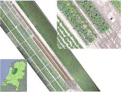
Figure 1 shows an image of the layout of an experimental field of the NAK in the central polder area of the Netherlands. During the experiment—which involved normal cultivation practices and varying weather conditions—all plants in the field were visually monitored several times by an experienced NAK inspector.
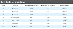
Table 1 shows varieties and infections used in the different rows of the field. Rows 1 through 3 contained plants infected with bacterial diseases, while rows 4 through 7 contained plants from 4 different varieties infected with the Potato Virus Y (PVY; genus Potyvirus, family Potyviridae) virus. Images of the plants in rows 1 through 3—which had mainly bacterial infections, some natural occasional Y virus infections, and some healthy plants—provided data for training a convolutional neural network (CNN). Plants in row 5 (Lady Claire) appeared to be 100% symptomatic and plants in row 4 (Rosa Gold) showed more than 95% symptomatic plants. Furthermore, Potato Virus X (PVX) symptoms on row 4 disturbed the manual scores of the crop experts, and the appearance of PVX was confirmed by a laboratory assay (ELISA). Therefore row 4 and 5 were excluded from hyperspectral analysis.
For capturing images, the team used an FX10 hyperspectral line scan camera from Specim (Oulu, Finland; www.specim.fi). Featuring a spectral range of 400 to 1000 nm, the camera has a CMOS sensor with image acquisition speed of up to 330 fps, and free wavelength selection from 224 bands within the camera coverage. Paired with the camera and connected via GigE interface for image acquisition was an NISE 3500 embedded PC from Nexcom (Taipei, Taiwan; www.nexcom.com), which features a Core i7/i5 processor from Intel (Santa Clara, CA, USA; www.intel.com).
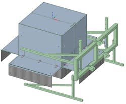
Light curtains placed around the measurement box blocked ambient light (Figure 2).
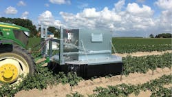
The measurement box was placed 3.1 m in front of a tractor that drove at a constant speed of 300 m / hour (0.08 m/s) during the measurements (Figure 3). The pushbroom line scan camera acquired images at 60 fps, resulting in an interval of 5 mm in the driving direction of the tractor.
To improve light sensitivity and speed, images were binned by a factor of two in the spatial direction and a factor for four in the spectral direction, resulting in line images of 512 x 56 pixels (Figure 4). As the bands at the start and end of the spectrum were noisy, only the central 35 bands were used for processing.
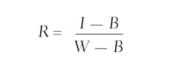
Thirteen DECOSTAR 51 PRO, 14-Watt, dichroic tungsten halogen lamps from Osram (Munich, Germany; www.osram.com) were placed in a row to provide even plant illumination. White and black references were taken at the start of each measurement cycle. The white reference object was a gray (RAL 7005) PVC plate, and the black reference was taken with the camera shutter closed. Reflection images were calculated by:
where I represents the raw hyperspectral Image, B the black reference, and W the white reference.
The total length of the crop rows were 110 m and 66 m for rows 1–3 and 4–7, respectively, with an interval of 5 mm, a total number of 22,000- and 13,200-line images per row were acquired.
Geo referencing
A crop expert visually inspected the plants in the experimental field to determine health status. Plants that showed Y-virus disease symptoms were geometrically stored with a real-time kinematic (RTK) global navigation satellite system (GNSS) rover, the HiPer Pro from TOPCON (Tokyo, Japan; www.global.topcon.com). A variable reluctance sensor (VRS) from 06-GPS (Sliedrecht, The Netherlands; www.06-gps.nl/english) ensured 0.02 m accuracy on the position estimate.
The crop expert obtained the position of a diseased plant by placing the rover at the center point of the plant. From the center point, a geometric plant polygon was constructed and stored for offline processing.
On each measurement day, the team obtained the real-world position of the hyperspectral line images using the tractor’s RTK-GNSS receiver, a Viper 4 from Raven Europe (Middenmeer, The Netherlands; www.raveneurope.com). These planar coordinates were rotated and scaled such that the crop rows were parallel in the X-direction. For each hyperspectral line, the system determined the health status by checking the intersection between the line and the geometric plant polygon. Lines that overlapped more than one polygon were left out of consideration.
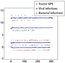
Figure 5 shows a plot of the GNSS positions of the RTK rover, labeled as viral or bacterial infection and the GNSS position of the tractor driving back and forth over the rows.
Deep learning methods
While CNNs typically classify entire images (label-per-image) or provide 2D segmentations (label-per-pixel), the team’s approach used a “weak” 1D label sequence in combination with a modified fully convolutional neural network (FCN), architecture to reduce the vast amounts of training data generally required.
The “weak” 1D label sequence has the advantage of increasing the effective number of labels (labels-per-line) available in the training set, thus lowering overfitting risk. The approach also substantially lowers the burden of labeling datasets. Instead of needing to provide pixel-level annotations, the researchers used GNSS locations of diseased individuals to generate ground truth on the line-level—a substantially simpler process.
The network used was an FCN with a non-standard decoder (final) portion. While the output for FCNs is usually a 2D segmentation, the researchers outputted a 1D segmentation with the goal of assigning a label to each line image. Because of imbalanced training data (a lot of healthier cases than diseased cases), the data was resampled to emphasize diseased examples. As deep learning needs a lot of training data, the available data was enriched by data augmentation techniques, such as random mirroring and rotation and randomized changes in image brightness.
FCNs suit semantic segmentation of 2D images, where one wants to assign a class (such as “human” or “dog”) to each pixel of the image. Employing only a combination of convolutions, pooling, unpooling and per-pixel operations (such as ReLU non-linear activation functions), FCNs produce a segmentation for the entire image in one forward pass, replicating the same computation for each region of the image.
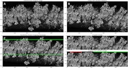
Constructed from 500 consecutive line images, each input image represents a subset of a row captured by the tractor. Each line image of 512 pixels retains 250 pixels. During testing, these represent the central 250 pixels, with the interval randomly chosen during training as a form of data enrichment. Figure 6 shows the process of generating a training or test image—with the annotation of the input images based on the health status of each potato plant as determined by the crop expert and stored with the (RTK-GNSS) rover. The top band indicates ground truth, with green and red labels indicating healthy or diseased plants, respectively. Black labels indicate regions excluded from testing due to labeling uncertainty. Input images have a resolution of 500 x 250. The number of feature maps at the input equals the number of hyperspectral bands kept (35).
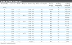
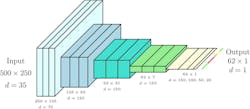
Described in Table 2, the network architecture shows a series of 17 stages, each of which contains a convolutional layer followed by optional layers such as max pooling, a per-element non-linearity (either Leaky ReLU activation functions with negative gradient of 0.01, or sigmoidal), batch normalization, and dropout (Figure 7).
A dropout probability of 0.5 was used. A SpatialDropout layer was used toward the start of the convolutional portion of the network (within stage 1). The fully-connected portion of the network (stages 14 through 16) uses standard dropout layers.
Stages 1 through 7 represent typical 2D FCNs. Here, a series of convolutions acting as successive feature extraction stages are performed. Interspersed max pooling stages lower the feature map resolution, allowing the convolutions to extract features based on larger regions of image context. The feature map spatial dimensionality reduces in a symmetrical fashion, leading to more enriched and discriminating features.
In Stages 8 through 13, the architecture departs from 2D FCNs in that pooling is restricted to the dimension parallel with individual line images. There were two sections (stages 8–10 and 11–13) containing three convolutions each, with both sections ending with a 1 x 4 max pooling, which had the effect of asymmetrically shrinking the feature map resolution from 62 x 31 to 62 x 7, and then finally 62 x 1. Referred to as “combiners,” these two stages combine evidence across a hyperspectral line (and its close neighbors) until the spatial dimension collapses to a length of 1. Additionally, the two sections shared the same parameters (Table 2), which was motivated by both these sections performing the operation of pooling evidence across local regions into larger regions.
Stages 14 through 17 performed the final per-label decision through a series of convolutions with 1 x 1 kernels. Due to the kernel dimensions, these were effectively fully-connected stages performed in parallel, and independently, on each output point. The final layer has a sigmoidal non-linearity, as the output should be a probability of disease.
The output layer produced 62 labels, while there were 500 pixels along the corresponding axis in the input image. Since each plant should occupy multiple sequential labels even at the lower resolution of the output, the team—concerned mainly with labeling entire plants as healthy or diseased—opted to forgo a trainable unpooling network in favor of a simple nearest neighbor upscaling to 500 pixels to match the input image.
Ground truth labeling involved use of GNSS coordinates of diseased plants as determined by crop experts. Training and testing the neural network requires labeling of each line image (either as diseased, healthy, or excluded). Initially, all line images were labeled as healthy. Then, for each diseased plant, the line image with GNSS tag closest to the diseased plant was located, which acted as a center point for subsequent labeling. The 150 line images before and after the center line were marked as excluded (if not already marked as diseased). Then, if the infection was specifically of a viral nature, the 50 line images before and after the center point were marked as diseased.
Because of non-uniformity in the dimensions and growth patterns of each plant, this procedure ensured only labeling regions with a high degree of certainty regarding the health of associated plants. Figure 6 shows an example of such a labeling, where a single plant with a viral infection is located toward the left-hand side of the image. The core diseased labels and excluded regions surround the plant, with regions marked as healthy extending beyond the excluded region.
Predictions for all line images in the input, regardless of labeling, were produced during training and testing. However, only lines with ground truth labeling as either healthy or diseased contributed to error measures used during training and evaluation of the system, whereas excluded lines did not contribute.
The model was trained on rows 2 and 3, with row 1 used as a validation set during training. After training, the resulting neural network was independently tested on rows 6 and 7. Used for training and testing was a system based on an Intel Xeon E5-1650 CPU with a 3.5 GHz clock speed and 16 Gb of RAM. Additionally, the system featured an NVIDIA GTX 1080 Ti GPU with 11 Gb of video memory. All data preprocessing, deep learning training, and validation was done with the PyTorch deep learning framework. At test time, a forward pass through the neural network took a total of 8.4 ms, of which 4.0 and 1.1 ms were the times taken to move data to and from the GPU, respectively.
Results
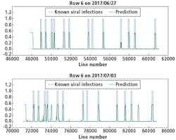
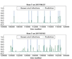
Although there were not many Y Virus-infected plants in the training set, the network performed well in predicting the infected plants in row 6 and 7 (Figures 8 and 9, respectively). In these figures, the x-axis shows the line number in the hyperspectral image of the total row.
The y-axis shows the output of the network as a probability.
An average of network predictions was calculated over all line images associated with a plant, and a probability threshold of 0.15 on the average distinguished the diseased plants for prediction (Figure 10).
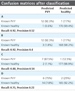
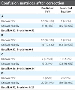
Table 3 provides the confusion matrices after classification for the different rows and measurement dates. From the confusion matrices, the precision (positive predictive value) and recall (sensitivity) were calculated, with precision a measure of the fraction of relative instances—the diseased plants among the retrieved instance—and recall the fraction of relevant instances retrieved over the total amount of relevant instances. Precision and recall are defined as:
where tp represents the true positive fraction, fp the false positive fraction, and fn the false negative fraction. For row 6, the precision is 0.52 and 0.4 for the first and second measurement week, respectively, and the recall is 0.92 for both weeks. For row 7, the precision measures are 0.54 and 0.23 and the recall is 0.88 and 0.75, respectively.
Investigation into the position of the FPs shows that most were connected to TPs. When ignoring the FPs connected to TPs, the confusion matrices are much better (Table 4). The recall measures stay the same, as this correction does not affect the FNs. The precision measures improve to 0.92 and 0.8 for row 6 and 0.78 and 0.3 for row 7, respectively.
Current practice involves manually scoring the plants in the field using a predefined protocol (NAK) of 40% of total plants scored. The accuracy of an experienced judge is 93%, but certified personnel need extensive field experience before becoming familiar with the symptoms induced by various pathogens in many potato varieties under different environmental conditions. Machine vision can detect disease symptoms with a precision close to the accuracy of an experienced crop expert, while also introducing the possibility of scanning the whole field compared to only 40%.
Despite limited training data, the prediction of PVY was successful. The percentage of detected infected plants, expressed in the recall values, is slightly lower (75–92%) than the accuracy of the crop expert (93%). Due to the low percentage of diseased plants, the precision values are worse, with a range from 0.23 to 0.54 (Table 3). Plants used as part of the research were already large and overlapping when the first imaging experiments started, so using smaller, non-overlapping plants should lead to improved accuracy of the position of the plant polygons and better performance overall. Furthermore, the independent test set consisted of plants from other cultivars than those in the training and validation sets. It is not expected that models will generalize well to new varieties as different growth patterns and surface characteristics may disturb regularities observed by the model specific to the training set cultivar.
However, the system obtained accuracies with precision larger than 0.75 for 3 out of 4 row/week combinations in the test set, indicating that the system has found real underlying regularities due to the disease state. Going forward, several challenges need to be addressed to use hyperspectral data in deep learning, including the size of the data and the noisiness of specific wavelength bands.
Gerrit Polder is a Senior Researcher at Wageningen University & Research (Wageningen, The Netherlands; www.wur.eu/agrofoodrobotics).
Related stories:
Spectral imaging system enables digital plant phenotyping
Multispectral and hyperspectral cameras expand the scope of industrial imaging
Share your vision-related news by contacting Dennis Scimeca, Associate Editor, Vision Systems Design
SUBSCRIBE TO OUR NEWSLETTERS
