The math behind Six Sigma metrics
By Valerie Bolhouse, Certified Six Sigma Blackbelt
(This information supports an article appearing in the January 2008 issue ofVision Systems Design, "Quality Numbers: Six Sigma.")
In nature and most manufacturing processes no two things are ever exactly the same. There exist small variations from part to part or measure to measure. If you were to acquire metrics on features of 100 "identical" parts and plot the values relative to frequency, you would be plotting a histogram. For stable processes, the curve would most likely be a normal, or bell-shaped, curve. The analysis of the data in this fashion is called descriptive statistics.
Data about the entire population is not usually studied. It is more useful to study a sample of that population and infer from the analysis what the entire population most likely looks like. This is inferential statistics. The confidence in the correctness of that prediction is dependent upon the size of the sample and the behavior of the data. Some of the useful characteristics that can be calculated from the data are described below.
The average value of the data is called the mean or X-bar. The equation for the mean is (X1+X2+X3+...+XN)/N, also denoted by ΣXi/N. Another measure calculated from the data is the variability, or the degree to which the individuals cluster about the mean. The most common measure of variability is the variance. The variance is calculated by squaring and summing the deviation of the individual data points from the mean. The equation for variance is s²=Σ (X )²/(N 1). The square root of the variance provides the standard deviation of the sample, s. If you have your data in an Excel spreadsheet, you can easily calculate the mean and standard deviation by using the built-in functions, AVE and STDEV.
The sample mean and standard deviation are used to estimate the population mean and standard deviation, which are denoted by the Greek letters μ and σ. The mean of the population is the central tendency of the data. The equation for the variance of the population is σ² = Σ(X-μ)²/ N, and the standard deviation, σ, is the square root of the variance.
The histogram can be made dimensionless for analysis by setting the mean to zero and scaling the units on the horizontal axis by dividing by the standard deviation. This is called the Z-Transform: Z = (point of interest--μ)/σ. This new plot is called a standard normal histogram. The normal distribution is completely described by its mean and standard deviation. The area under the curve represents 100% of the possible observations. The curve is symmetrical about the mean, and the tails extend to infinity. The area under the distribution curve also represents the probability. You can evaluate the probability of your manufacturing distribution falling outside of the specification limit, or predict the failure rate or yield by evaluating where the specification limit is set relative to the Z-score.
The area under the curve bounded by ±1σ contains 68.26% of the total population, while ±2σ has 95.44% and ±3σ has 99.73%. If the upper and lower specification limits were set at ±3σ, then 99.73% of the product would fall within specification and .27% falls outside of the limits. If 1,000,000 parts were manufactured with this process capability, then you would expect 2700 defective parts. This would be a 3σ process. Three sigma used to be the standard for high-quality manufacturing, but that is no longer true in today's competitive market.
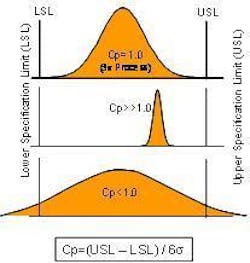
Six sigma is the new standard. If you calculate the area under the curve outside of ±6σ, you would see that it produces two defects per billion—-not million! Since this is not feasible or cost justifiable in most instances, Six Sigma uses a more pragmatic definition of 3.4 defects per million. It assumes that process variability will stay constant over time at ±4.5σ, but you will see a shift in the process mean of up to ±1.5σ. This is realistic in most manufacturing processes. If you are drilling a hole, the diameter might not vary widely, but it is likely that the location of the hole might move over time due to fixturing tolerances or machine wear. Or if you are painting or printing, the color might shift over time, but within the lot, the color itself will remain stable (see figures above).
Six Sigma metrics include both short-term and long-term capability. Short-term capability is measured during runoff for machine acceptance, or during the process validation phase. A small sample of parts are run, and plus or minus six standard deviations of the measured variability should be within the specification limits. It is expected that over time, the long term capability will have process variation of no more than ±4.5σ with a ±1.5σ mean shift.
Process potential
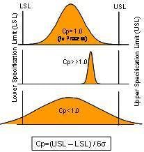
If a process is stable and in control, the variability can be graphed in a histogram plot, and ±3 standard deviations will fall within the upper and lower specification limits. There is a statistical metric for assessing process potential, or Cp, which relates the system tolerance to process variation (standard deviation). The equation for Cp is Cp = (USL-LSL)/6σ. Therefore, a 3 σ process, which is ±3σ for a total of six standard deviations, has a Cp of 1.0, and a 6 σ process has a Cp of 2.0. Cp tells you if your system variability falls within the tolerances for the specification. If you can't get the process to be repeatable within the tolerance set by the specification limits, no amount of tweaking will ever get you to where you can reliability make good parts. This is why Cp is termed process potential (see figure below).
Process capability
You also need to be concerned with centering—the mean of your process distribution should be centered about the target specification. This is process capability, or Cpk. Cpk is the lesser of: (USL--mean)/3σ and (mean--LSL)/3σ. If you have good process potential (repeatability), calibration or set-up is usually all that is required to also have good process capability.
An analogy often used to describe these metrics is parking a car in the garage. The width of the car represents the process tolerance and the garage door opening represents the specification limits. If the car is bigger than the garage door (process variation larger than specification), it is not possible to park the car in the garage without hitting one or both sides with every attempt. However, even if the car is smaller than the garage door, you still must be centered in order to not bump into one of the specification limits.
There are many other distributions and metrics used by practitioners of Six Sigma. The binomial distribution is used for attribute analysis to determine the proportion of defective units in a lot. The Poisson distribution is similar except that it is used for the average rate of occurrence of defects, such as the number of paint defects per square foot of surface area. The type of distribution used should match the data being analyzed.
Descriptive and inferential statistics are the foundation of Six Sigma. The Six Sigma program employs a practical, disciplined approach to collecting and analyzing data in order to understand and improve process capability by reducing variability. Performance, capability, and improvement can all be quantitatively described by the common language of statistics.
